
Most formula transformations can be done using value source formulas, but the report designer tool also supports using literal Excel style formulas.
While value source formulas are evaluated before populating a cell, Excel style formulas of this type are evaluated afterwards. The report designer supports a subset of the Excel formula language, along with helpers to generate references to other cells.
There are limited times when you might want to use an Excel style formula:
- You want to export the report to Excel and manually change numbers within the report. The Excel style formula values will automatically update as you edit the report.
- You use totals which are based on ratios (i.e. percentages).
For more information on the differences you can read this dedicated article.
Creating Excel Style Formulas
Excel style formulas are entered into the value source formula area for a column. To change to Excel style formula mode, start the value source formula with an equals sign. For example: =1 + 2
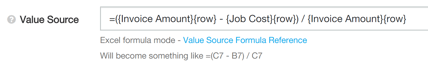
When you enter an Excel style formula, the report designer will change to show a preview of the formula as it will appear in the spreadsheet. This is useful, as Excel style formulas can appear complex before transformed.
You can always check how Wink transforms your formula by exporting the report the Excel and looking at the cell contents:
![]()
If there is a mistake in your formula (e.g. incorrect spelling, or a function Wink doesn't support) the report will show #NAME? in that cell. This is the same behaviour as Excel.
Cell References
When working in Excel, you can reference other cells by name. For example: =A7 * B7
This method doesn't work so well for reports because column letters change as we drag columns around, and row numbers change for each row in the report. Instead the report designer supports using curly braces to reference columns and rows.
For example: a formula for profit might look like ={Invoice Amount}{row} - {Job Cost}{row}. When placed into the report, this will become =C7 - B7 for the first report row, =C8 - B8 for the second report row, and so on.
Columns
Column references use the title of other columns in the report. If you rename a column in the report, any formulas which reference that column will update to reflect the new column title.
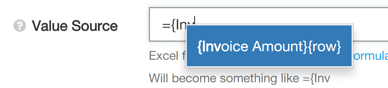
When you type an open curly brace, the report designer will help you auto-complete the column reference. It is recommended to use the suggested values, as the formula will be invalid if there is a spelling mistake (including capitalisation!).
Rows
The most common row reference is to use the current row: {row}
Also valid are {prev_row} and {next_row}, and grouping total formulas can make use of {first_row} and {last_row}.
To make a running total, you can do something like ={Line Total}{row} + {Running Total}{prev_row} .
Functions
A subset of the Excel formula functions are available.
| Function | Examples | Notes |
|---|---|---|
| SUM(cell_or_range_1, cell_or_range_n, ...) | SUM({Line Total}{first_row}:{Line Total}{last_row}) | Add up all the cell values. |
| COUNT(range) | COUNT({Line Total}{first_row}:{Line Total}{last_row}) | Count the number of values in the range. Blank cells are ignored. |
| AVERAGE(range) | AVERAGE({Line Total}{first_row}:{Line Total}{last_row}) | Average of cell values. Blank cells are ignored. |
| MAX(cell_or_range_1, cell_or_range_n, ...) | MAX({Line Total}{first_row}:{Line Total}{last_row}) MAX({Quote Amount}{row},{Invoice Amount}{row}) |
Find the maximum value in the provided ranges. |
| MIN(cell_or_range_1, cell_or_range_n, ...) | MIN({Line Total}{first_row}:{Line Total}{last_row}) MIN({Quote Amount}{row},{Invoice Amount}{row}) |
Find the minimum value in the provided ranges. |
| MOD(value, divisor) | MOD({row}, 2) | Calculate the remainder of integer division. Useful for alternating rows. |
| IF(condition, true_value, false_value) | IF({Category}{row} = "Special", {Total}{row} * 2, {Total}{row}) | As per Excel IF. |
| NOT(expression) | NOT({Category}{row} = "Special") | Reverse a true/false value. |
| AND(expression_1, expression_n, ...) | AND({Category}{row} = "Special", {Total}{row} > 100) | True if all expressions provided are true. |
| OR(expression_1, expression_n, ...) | OR({Category}{row} = "Special", {Category}{row} = "Normal") | True if any expressions provided are true. |
| ABS(value) | ABS(-1) | Absolute value, discard any negative signs |
| SQRT(value) | SQRT(9) | Square root |
| ISERROR(expression) | ISERROR(10 / 0) | True if <expression> produces an error |
| IFERROR(expression, value) | IFERROR(10 / 0, 0) | Returns <value> if <expression> produces an error |
| DATEVALUE(text_value) | DATEVALUE("2010-05-31") DATEVALUE("1/1/18") DATEVALUE({Text Column}{row}) |
Convert the text string <text_value> into a date if possible. |
Use In Grouping Totals
The most common use of Excel style formulas is for percentage formulas in grouping totals.
Consider a report which has columns Labour Cost and Invoice Value, and we want to show Cost as a percentage of Invoice Value.
The Excel style formula to calculate this would be =IFERROR({Labour Cost}{row} / {Invoice Value}{row} , 0)
For the total row, it needs to be a similar calculation but for the totals of each of Labour Cost and Invoice Value. This can be done by selecting Formula for the total row option:
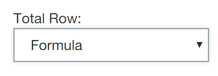
This option only appears when the value source formula is an Excel style formula (i.e. starts with an equals sign).
Be sure to set the total row to Sum for Labour Cost and Invoice Value.